pandas
Excel is a grid of cells that can hold anything — a number, a date, a piece of text, a blank. You can sort one column, filter the whole sheet by a condition, or add a new column that is a formula over two others. What Excel cannot do is script. Every click is a click. Every filter has to be reapplied when the data refreshes. pandas is Excel rewritten as Python. Every sheet is a DataFrame, every column is a Series, every filter and group and merge is a function call you can save in a file and rerun tomorrow on tomorrow's data.
The library was born out of a frustration at a hedge fund. In 2008 a graduate of MIT named Wes McKinney was at AQR Capital, a quant firm whose models lived in R and whose production lived in Excel. R handled DataFrames well but was miserable for general-purpose code. Python handled general-purpose code well but had nothing DataFrame-shaped in its standard library. McKinney started writing pandas on nights and weekends, open-sourced it in 2009, and left AQR to work on it full time. By 2012 it was the default tool for financial analysts who wanted their work to outlive the month. The big rewrite came in 2023 with pandas 2.0, which swapped the internal memory layout from NumPy to Apache Arrow. Arrow stores columns the way a database stores them, which means pandas can now hand a zero-copy reference to a column directly to DuckDB, Polars, or Spark. Same API, same DataFrame, different engine under the hood.
Install pandas. This lesson works with an NBA box-score dataset — about 2,400 games per regular season, 30 teams, roughly 20 columns per row. The public mirror hosted on GitHub by Nathan Lauga has every game since 2004. The raw file has more columns than we need; this lesson uses a trimmed version for clarity. Write the CSV out by hand so the lesson runs offline and every reader sees the same numbers.
cd ~/learning-python
source .venv/bin/activate
pip install pandas
mkdir nba
cd nba
touch games.csv
touch explore.py
cd $HOME\learning-python
.venv\Scripts\Activate.ps1
pip install pandas
mkdir nba
cd nba
ni games.csv
ni explore.pyOpen games.csv and paste 16 rows — four teams, four games each, winners and losers recorded as plain numbers. This is a deliberately small slice so you can check every aggregation by hand:
date,home_team,away_team,home_pts,away_pts,home_fg_pct,home_ast,home_reb
2024-11-01,LAL,GSW,118,104,0.48,26,44
2024-11-02,LAL,DEN,103,110,0.42,22,41
2024-11-04,LAL,BOS,99,105,0.41,20,38
2024-11-06,LAL,GSW,112,108,0.46,28,43
2024-11-01,GSW,LAL,104,118,0.44,24,40
2024-11-03,GSW,BOS,121,113,0.51,30,46
2024-11-05,GSW,DEN,115,109,0.49,27,42
2024-11-07,GSW,BOS,107,115,0.43,21,39
2024-11-02,DEN,LAL,110,103,0.50,29,48
2024-11-04,DEN,BOS,98,101,0.44,23,45
2024-11-05,DEN,GSW,109,115,0.45,25,44
2024-11-07,DEN,LAL,114,108,0.52,31,47
2024-11-01,BOS,DEN,119,104,0.53,28,42
2024-11-03,BOS,GSW,113,121,0.47,22,40
2024-11-06,BOS,LAL,105,99,0.50,26,41
2024-11-08,BOS,DEN,101,98,0.46,24,43
Now explore the data. Open explore.py and start with a read:
import pandas as pd

games = pd.read_csv("games.csv", parse_dates=["date"])
print(games.head())
print()
print("shape:", games.shape)
print("dtypes:")
print(games.dtypes)
date home_team away_team home_pts away_pts home_fg_pct home_ast home_reb
0 2024-11-01 LAL GSW 118 104 0.48 26 44
1 2024-11-02 LAL DEN 103 110 0.42 22 41
2 2024-11-04 LAL BOS 99 105 0.41 20 38
3 2024-11-06 LAL GSW 112 108 0.46 28 43
4 2024-11-01 GSW LAL 104 118 0.44 24 40
shape: (16, 8)
dtypes:
date datetime64[ns]
home_team object
away_team object
home_pts int64
away_pts int64
home_fg_pct float64
home_ast int64
home_reb int64
dtype: objectread_csv inferred every column's type. Numbers became int64 or float64. Text became object, which is pandas for "a column of Python strings." The parse_dates argument turned the date column from text into a proper datetime64, which means you can filter by month or sort by day without reparsing. .head() shows the first 5 rows; .tail() the last 5; .shape is (rows, columns) the same way NumPy reports it.
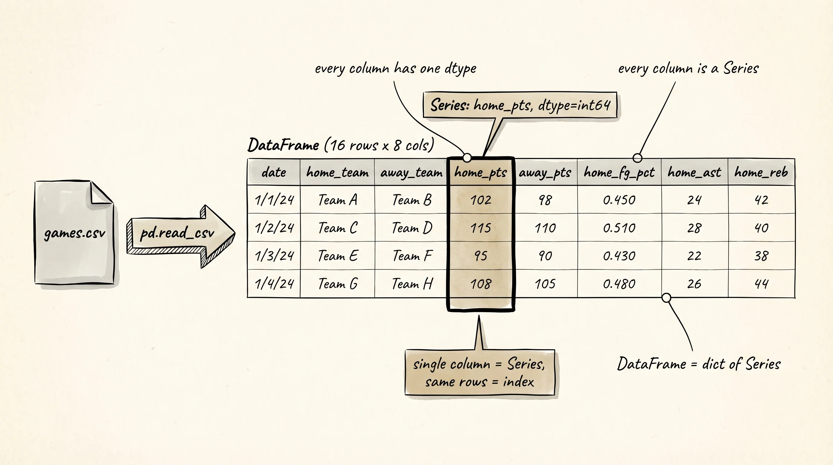
A DataFrame is a dictionary of Series. A Series is a named, typed column. Pull one out:
print(type(games["home_pts"]))
print(games["home_pts"].describe())
<class 'pandas.core.series.Series'>
count 16.000000
mean 109.125000
std 7.326787
min 98.000000
25% 103.750000
50% 109.500000
75% 114.250000
max 121.000000
Name: home_pts, dtype: float64.describe() is the one function to memorize first. It gives you count, mean, standard deviation, min, quartiles, and max in one call. Run it on a DataFrame and it runs on every numeric column. Run it on a Series and it runs on one column. Every number above was computed in C over the 16 rows.
Filtering reads like English. Give pandas a boolean Series the same length as the DataFrame and it keeps the rows where the boolean is True:
blowouts = games[games["home_pts"] - games["away_pts"] >= 10]
print(blowouts[["date", "home_team", "away_team", "home_pts", "away_pts"]])
date home_team away_team home_pts away_pts
0 2024-11-01 LAL GSW 118 104
5 2024-11-03 GSW BOS 121 113
8 2024-11-02 DEN LAL 110 103
12 2024-11-01 BOS DEN 119 104Four games where the home team won by 10 or more. The expression games["home_pts"] - games["away_pts"] >= 10 returns a boolean Series. The outer brackets take only the True rows. The last brackets project 5 columns for a readable print. Combine conditions with & (and) and | (or). Parentheses are required because & binds tighter than >=:
lal_wins = games[(games["home_team"] == "LAL") & (games["home_pts"] > games["away_pts"])]
print(lal_wins[["date", "home_team", "away_team", "home_pts", "away_pts"]])
date home_team away_team home_pts away_pts
0 2024-11-01 LAL GSW 118 104
3 2024-11-06 LAL GSW 112 108Two Lakers home wins against the Warriors. The condition chain mirrors the SQL WHERE home_team = 'LAL' AND home_pts > away_pts in exactly the same number of characters.
Groupby is where pandas earns its place as the default data tool. Grouping splits the DataFrame into buckets based on a column value and applies an aggregation to each bucket. Average home points per team, a one-line question:
home_avg = games.groupby("home_team")["home_pts"].mean()
print(home_avg)
home_team
BOS 109.50
DEN 105.25
GSW 111.75
LAL 108.00
Name: home_pts, dtype: float64The Warriors score the most at home in this slice; the Nuggets the least. One function call, four buckets, four averages. You can aggregate multiple columns with different functions in one call using .agg:
summary = games.groupby("home_team").agg(
    games_played=("home_pts", "count"),
    avg_pts=("home_pts", "mean"),
    max_pts=("home_pts", "max"),
    avg_fg_pct=("home_fg_pct", "mean"),
    avg_ast=("home_ast", "mean"),
)
print(summary)
games_played avg_pts max_pts avg_fg_pct avg_ast
home_team
BOS 4 109.50 119 0.490 25.0
DEN 4 105.25 114 0.478 27.0
GSW 4 111.75 121 0.468 25.5
LAL 4 108.00 118 0.442 24.0Every row is a team. Every column is an aggregation. Read that table top to bottom and you know more about this slice of the season than you did 30 seconds ago. A question worth asking from the table: the Warriors have the highest max (121) but the lowest avg_fg_pct. How?
Two answers tie together. First, the Warriors are a high-volume three-point team in real life and in this slice — more shots per game means more total points even at a lower make rate. Second, a max of 121 is a single game. An average over 4 games hides the variance. Pandas will tell you the variance too: .agg(std_pts=("home_pts", "std")) gives you a standard deviation column and the Warriors sit at 7.85 points, the highest spread in the table.

A second groupby shape worth seeing: a pivot. The raw data has one row per game. If you want a table where rows are home teams, columns are away teams, and cells are the average points scored by the home team against that away team, pivot_table does it:
pivot = games.pivot_table(
    index="home_team",
    columns="away_team",
    values="home_pts",
    aggfunc="mean",
)
print(pivot)
away_team BOS DEN GSW LAL
home_team
BOS NaN 110.0 113.0 105.0
DEN 98.0 NaN 109.0 112.0
GSW 114.0 115.0 NaN NaN
LAL 99.0 103.0 115.0 NaNThe diagonal is NaN because nobody plays themselves. Any other NaN means that matchup did not happen in this slice. Pandas handles missing data gracefully — NaN is pandas' word for "no value." Every numeric aggregation skips NaN by default. If you want a 0 in those slots, fill with .fillna(0).
Merging is how pandas joins two DataFrames on a shared column. Say you have a second CSV with each team's win total for the season. Build it inline to keep the lesson self-contained:
standings = pd.DataFrame({
    "team": ["LAL", "GSW", "DEN", "BOS"],
    "wins": [48, 52, 57, 64],
})

merged = games.merge(standings, left_on="home_team", right_on="team", how="left")
print(merged[["date", "home_team", "home_pts", "wins"]].head())
date home_team home_pts wins
0 2024-11-01 LAL 118 48
1 2024-11-02 LAL 103 48
2 2024-11-04 LAL 99 48
3 2024-11-06 LAL 112 48
4 2024-11-01 GSW 104 52Every row now carries the season-long win total for the home team. how="left" keeps every row from the left DataFrame even if the right has no match; how="inner" drops unmatched rows; how="outer" keeps everything from both sides and fills gaps with NaN. The vocabulary matches SQL joins because pandas was designed by someone who reached for SQL first and found it missing from Python.
This lesson does no plotting. The NBA DataFrame is the material the next lesson turns into a chart. pandas has a built-in .plot() that wraps matplotlib, and you can use it for a quick sanity check when you are typing at the REPL, but a published chart wants a library built from the ground up for a reader looking at a screen. The next lesson is that library.