NumPy

A spreadsheet is a grid of numbers a human can scroll through. NumPy is that grid, with two changes. The first is that the grid lives in one flat block of memory instead of a scattered Python list of objects, so the CPU can walk it the way it walks a row of houses on a straight street. The second is that every operation on the grid — adding 1 to every cell, multiplying one column by another, summing a million values — runs inside C code compiled decades ago to go as fast as the machine allows. A NumPy array is a spreadsheet that runs at the speed of a C program.

Scientific Python in the 1990s was a standoff between two competing array libraries. Numeric came out of Lawrence Livermore in 1995. Numarray came out of the Space Telescope Science Institute in 2001. Both stored arrays. Neither talked to the other. Every scientific package had to pick a side, and half the ecosystem ran on the wrong library. A mathematician at Brigham Young University named Travis Oliphant spent 2005 writing a third library that merged the two, kept the good parts of each, and shipped it as NumPy in 2006. By 2010 every serious Python science project was built on it. In 2020 a paper in Nature listed NumPy as the foundation for the gravitational-wave detection at LIGO and the first image of a black hole from the Event Horizon Telescope. The grid won.

Install the library into the venv you have been using and start a fresh file.

cd ~/learning-python
source .venv/bin/activate
pip install numpy
touch numpy_intro.py

cd $HOME\learning-python
.venv\Scripts\Activate.ps1
pip install numpy
ni numpy_intro.py

A NumPy array starts as a regular Python list handed to np.array. Open numpy_intro.py and watch what the library does with four numbers:

import numpy as np
 
row = np.array([10, 20, 30, 40])
print("array:  ", row)
print("shape:  ", row.shape)
print("dtype:  ", row.dtype)
print("nbytes: ", row.nbytes)
print("strides:", row.strides)

Output:

array:   [10 20 30 40]
shape:   (4,)
dtype:   int64
nbytes:  32
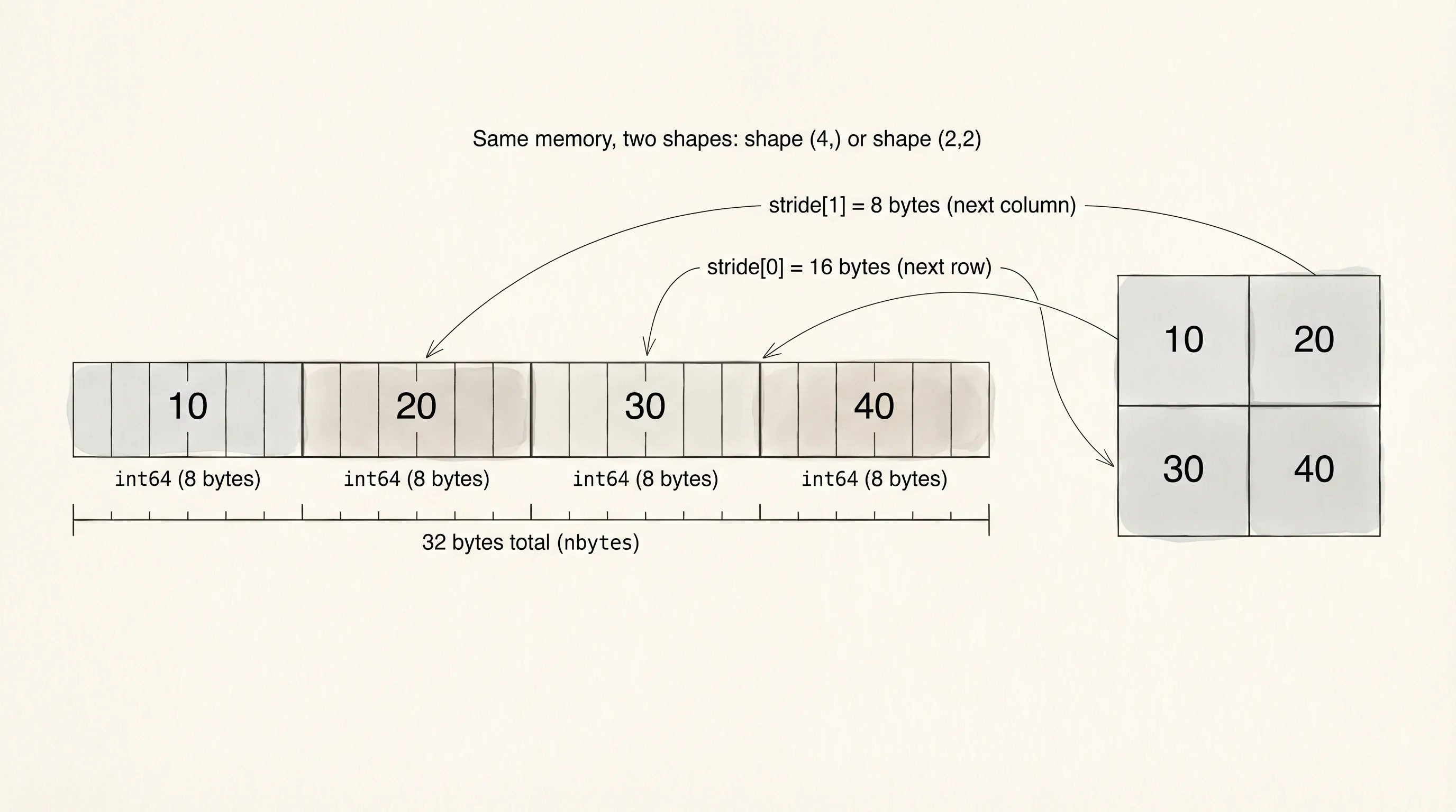
strides: (8,)

The dtype says every cell is an int64, which is 8 bytes wide. Four cells times 8 bytes per cell is 32 bytes, and that is exactly what nbytes reports. A Python list holding the same four integers would take 8 pointers plus 4 heap-allocated int objects plus the list header, roughly 140 bytes, and every walk of the list has to follow every pointer to find the actual value. The NumPy array holds the values themselves, back to back, with zero indirection. strides tells you how many bytes to skip to get from one cell to the next: 8. That is the shape of a fast loop.

A 2D grid stores exactly the same way. Reshape the four-element row into a 2x2 square:

grid = row.reshape(2, 2)
print(grid)
print("shape:  ", grid.shape)
print("strides:", grid.strides)

[[10 20]
 [30 40]]
shape:   (2, 2)
strides: (16, 8)

Same 32 bytes. Same four integers. The shape became (2, 2). The strides became (16, 8) — move 16 bytes to get to the next row, 8 bytes to get to the next column. Reshaping did not copy anything; NumPy changed its interpretation of the same memory block. That is why reshape runs in a microsecond on a gigabyte of data.

Vectorization is the word for "let the library run the loop in C." Adding 1 to every cell in a Python list takes a for loop. Adding 1 to every cell in a NumPy array takes one operator:

print(row + 1)
print(row * 2)
print(row ** 2)

[11 21 31 41]
[20 40 60 80]
[ 100  400  900 1600]

Three operations, each traversing every cell. No explicit loop anywhere. The library recognizes +, *, and ** on arrays and dispatches to a compiled function that walks the memory block and fills a new array with the result. The speed difference is not small. Write a benchmark that compares Python's built-in sum over a million integers to NumPy's np.sum over the same million. Save this to a file called bench_sum.py:

import time
import numpy as np
 
N = 1_000_000
py_list = list(range(N))
np_array = np.arange(N, dtype=np.int64)
 
start = time.perf_counter()
py_total = sum(py_list)
py_seconds = time.perf_counter() - start
 
start = time.perf_counter()
np_total = int(np.sum(np_array))
np_seconds = time.perf_counter() - start
 
print(f"python sum: {py_total:>12,} in {py_seconds * 1000:.2f} ms")
print(f"numpy  sum: {np_total:>12,} in {np_seconds * 1000:.2f} ms")
print(f"speedup:    {py_seconds / np_seconds:.0f}x")

A representative run on a recent laptop:

python sum:  499,999,500,000 in 8.42 ms
numpy  sum:  499,999,500,000 in 0.34 ms
speedup:    25x

Same answer, 25 times faster. Every CPython bytecode instruction takes about 50 nanoseconds to dispatch. A million of them take 50 milliseconds, before the integer add even happens. np.sum skips that dispatch — one call into C, one tight loop in registers, one return. The bigger the array, the wider the gap grows.

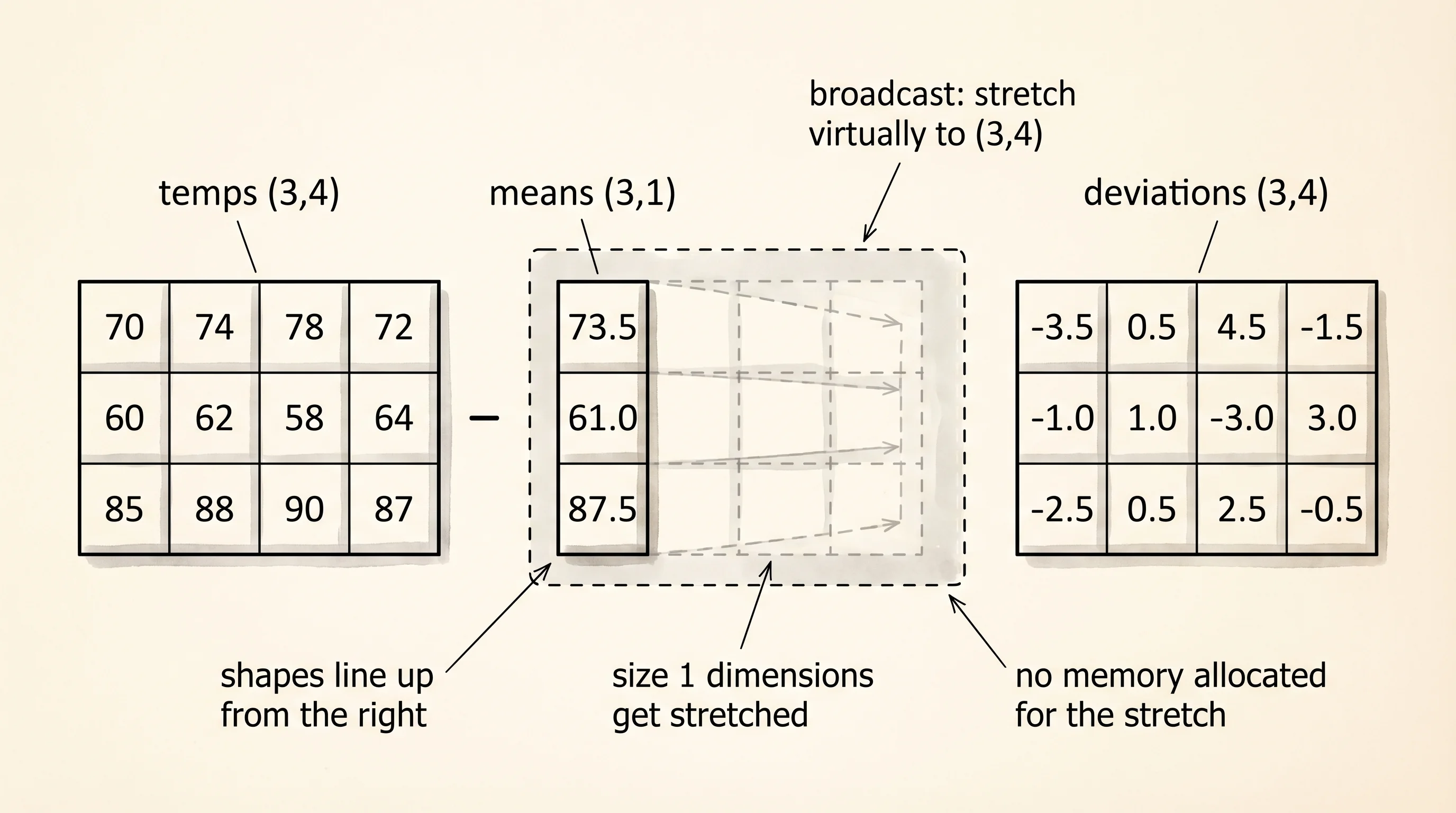
Broadcasting is the second trick NumPy gives you for free. Broadcasting means a small array can line itself up against a bigger array without you writing a loop to match shapes. Say you have the temperatures of 3 cities over 4 days, shape (3, 4), and you want to subtract each city's mean from its row. A city mean array is shape (3,). A Python solution reaches for a nested loop. NumPy reads the shapes and does it in one line:

temps = np.array([
    [70, 74, 78, 72],
    [60, 62, 58, 64],
    [85, 88, 90, 87],
])
means = temps.mean(axis=1, keepdims=True)
print("means:")
print(means)
print("deviations:")
print(temps - means)

means:
[[73.5]
 [61. ]
 [87.5]]
deviations:
[[-3.5  0.5  4.5 -1.5]
 [-1.   1.  -3.   3. ]
 [-2.5  0.5  2.5 -0.5]]

The mean call with axis=1 collapses each row to a single value, producing a (3, 1) column. The subtraction sees a (3, 4) on the left and a (3, 1) on the right, and NumPy stretches the column across all 4 days for the subtraction. No loop. No new memory for the stretched column — the library treats the one column as if it were copied 4 times, without actually copying.

Now the hands-on piece the curriculum asked for. Every algorithm in the data-structures section rewrote itself from primitives to a library version. Fibonacci is the cleanest example, because the recursive version has an exponential call tree and the loop version writes one line of Python per number. NumPy can compute the first N Fibonacci numbers with one matrix power. The math trick is that multiplying the matrix [[1, 1], [1, 0]] by itself n times produces [[F(n+1), F(n)], [F(n), F(n-1)]]. Read that identity once and write it into code:

import numpy as np
 
 
def fib_numpy(n: int) -> np.ndarray:
    matrix = np.array([[1, 1], [1, 0]], dtype=object)
    result = np.zeros(n + 1, dtype=object)
    result[0] = 0
    result[1] = 1
    current = np.array([[1, 1], [1, 0]], dtype=object)
    for i in range(2, n + 1):
        current = current @ matrix
        result[i] = int(current[0, 1])
    return result
 
 
print(fib_numpy(12))

[0 1 1 2 3 5 8 13 21 34 55 89 144]

The dtype=object keeps Python's arbitrary-precision integers inside the array, because Fibonacci numbers outgrow int64 around position 93. The @ operator is Python's matrix-multiply operator, added in Python 3.5 specifically so NumPy users did not need a verb for it. Every iteration folds one more matrix into current, and the top-right cell of the product is the next Fibonacci number. The outer array result collects them in order.

A question worth answering from the output: if the matrix trick is one line, why does the loop run n - 1 times?

Because the matrix trick computes F(n) for a given n, not the whole sequence at once. To print the first 12 Fibonacci numbers in order you still need to walk i from 2 to 12. The win is not "no loop." The win is "each iteration is a matrix multiply in C." For a single giant Fibonacci — the 10,000th number — you would skip the loop and use fast exponentiation (matrix ** n using repeated squaring) to jump to the answer in log n multiplications. Same library, same @ operator.

Slicing a NumPy array returns a view, not a copy. A view is a pointer into the same memory block with a different shape and stride interpretation. Mutations through a view rewrite the original array, which is the single biggest footgun in the library. Prove it to yourself:

grid = np.arange(12).reshape(3, 4)
print("original:")
print(grid)
row_two = grid[1]
row_two[:] = 99
print("after mutating row_two:")
print(grid)

original:
[[ 0  1  2  3]
 [ 4  5  6  7]
 [ 8  9 10 11]]
after mutating row_two:
[[ 0  1  2  3]
 [99 99 99 99]
 [ 8  9 10 11]]

row_two is not a new array. It is a 4-element window into the same 48 bytes that grid occupies. Assign into the view, the window writes straight into the shared memory, and the original grid changes. The fix when you want a real copy is row_two = grid[1].copy(). This is the price of zero-copy slicing; every serious NumPy programmer has been bitten by it once.

NumPy is fast because every cell has the same type and every cell sits next to the next one. That fixed-size row-and-column shape is exactly what breaks when real data shows up. A CSV of NBA games has numbers in some columns, strings in others, dates in a third, and a sprinkle of missing cells. The next lesson reaches for a library built to handle the mess that a NumPy array refuses to store.