Statistics You Actually Need

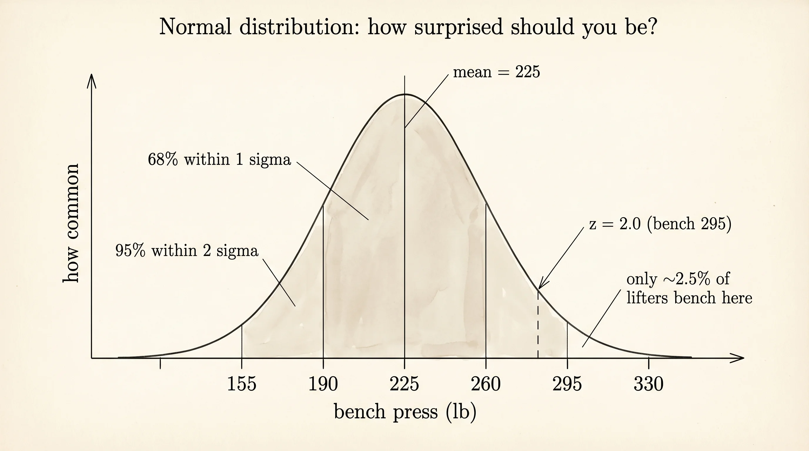
A guy walks into a gym and benches 225. How surprised should you be? At a commercial gym on a Saturday morning, not much — half the guys in the room are doing the same. At a retirement home, you just saw a miracle. The number 225 did not change. The distribution around it did. Statistics is the math for answering "how surprised should I be" with a number instead of a shrug, and every tool in this lesson is a different way of sizing up the room before you judge the lift.

The math came out of practical problems. In 1763 a Presbyterian minister named Thomas Bayes wrote an essay on how to update your belief about a coin when you see it land heads a few times — published after he died. In the 1810s Carl Friedrich Gauss worked out the shape now called the normal distribution while tracking errors in astronomical measurements at the Göttingen observatory. The modern p-value came from Ronald Fisher at Rothamsted, an agricultural research station north of London, in the 1920s. Fisher was tired of farmers arguing whether a new fertilizer actually increased yield or the field just had a good year. He needed a number that said: if the fertilizer did nothing, how often would a crop look this good by luck? That question became the p-value, and it has held up for 100 years despite a replication crisis in the 2010s that caught thousands of published studies using it wrong.

The warehouse from the last lesson holds the data. Every track has a tempo, a danceability score between 0 and 1, an energy score, and an explicit flag. Connect to it from a new file called stats.py and pull the numbers out.

import sqlite3
from pathlib import Path
 
connection = sqlite3.connect(Path("warehouse.db"))
cursor = connection.cursor()
cursor.execute("SELECT tempo FROM tracks WHERE tempo > 0")
tempos = [row[0] for row in cursor.fetchall()]
print("tracks:", len(tempos))
print("first five tempos:", tempos[:5])

tracks: 169125
first five tempos: [118.469, 83.972, 80.922, 64.678, 114.088]

The mean is the flat average — add everything and divide by the count. The variance is the average of the squared gaps from the mean, which punishes big misses more than small ones. The standard deviation is the square root of the variance, which puts the number back into the same units as the original data. For a gym full of 225-pound benchers, the mean is 225, the standard deviation might be 35, and a guy benching 295 is two standard deviations above the room. That is roughly how often in a bell-curve-shaped crowd you would see such a lift: a little under 3 percent of the time.

import math
 
n = len(tempos)
mean_tempo = sum(tempos) / n
variance = sum((t - mean_tempo) ** 2 for t in tempos) / n
std_dev = math.sqrt(variance)
 
print("mean tempo:", round(mean_tempo, 2))
print("standard deviation:", round(std_dev, 2))
print("a 180-BPM song is", round((180 - mean_tempo) / std_dev, 2), "standard deviations above the mean")

mean tempo: 117.6
standard deviation: 30.71
a 180-BPM song is 2.03 standard deviations above the mean

The number 2.03 is a z-score — how many standard deviations a value sits from the mean. A z-score of 2 is the line many fields use to call something surprising. A z-score of 3 is the line particle physics used to announce the Higgs boson discovery in 2012, adjusted for the fact that they were looking at billions of collisions and needed a much stricter threshold to avoid false alarms.

The mean is an estimate. You only measured 169,125 tracks, not every song ever recorded. If the dataset had sampled a different 169,125 you would have gotten a slightly different mean. How wide is that wiggle? A confidence interval is the answer. You resample the data thousands of times with replacement — a technique called the bootstrap, invented by Stanford statistician Bradley Efron in 1979 — and look at how much the mean jumps around. The 95 percent confidence interval is the range that contains the middle 95 percent of those resampled means.

import random
 
random.seed(42)
 
def bootstrap_mean_ci(values, rounds=1000):
    n = len(values)
    means = []
    for _ in range(rounds):
        sample = [values[random.randrange(n)] for _ in range(n)]
        means.append(sum(sample) / n)
    means.sort()
    lo = means[int(rounds * 0.025)]
    hi = means[int(rounds * 0.975)]
    return lo, hi
 
subset = tempos[:5000]
lo, hi = bootstrap_mean_ci(subset, rounds=500)
print("mean of 5000 tracks:", round(sum(subset) / len(subset), 3))
print("95% confidence interval:", (round(lo, 3), round(hi, 3)))

mean of 5000 tracks: 112.548
95% confidence interval: (111.719, 113.416)

The interval says that if you grabbed another 5,000 tracks at random from the same universe, the mean tempo would land between 111.7 and 113.4 BPM about 95 times out of 100. The number you measured is not a single point — it is a range. A bigger sample would tighten the range.

That tightening is the Central Limit Theorem at work. Pierre-Simon Laplace sketched it in 1810 and mathematicians cleaned it up over the next century. The claim is strange at first. You can take samples from any shape of distribution — a lumpy one, a skewed one, a totally chaotic one — and if you take the mean of each sample and plot those means, the plot always drifts toward a bell curve. The individual songs do not have to be normal. The average of a bunch of songs does. Watch it happen.

import random
import collections
 
def histogram(values, bins=20):
    lo = min(values)
    hi = max(values)
    step = (hi - lo) / bins
    counts = [0] * bins
    for v in values:
        idx = min(int((v - lo) / step), bins - 1)
        counts[idx] += 1
    return counts
 
def draw(counts):
    top = max(counts)
    for count in counts:
        bar = "#" * int(count / top * 40)
        print(f"{count:4d} | {bar}")
 
random.seed(7)
for sample_size in [2, 10, 50]:
    sample_means = []
    for _ in range(2000):
        sample = [random.choice(tempos) for _ in range(sample_size)]
        sample_means.append(sum(sample) / sample_size)
    print(f"\nsample size = {sample_size}")
    draw(histogram(sample_means))

sample size = 2
  14 | #
  35 | ##
  58 | ###
  92 | #####
 138 | ########
 189 | ###########
 231 | #############
 275 | ################
 298 | #################
 271 | ###############
 194 | ###########
 130 | #######
  76 | ####
  ...
 
sample size = 10
   2 |
   6 |
  21 | #
  60 | ####
 144 | ##########
 264 | ###################
 389 | ############################
 441 | ################################
 324 | #######################
 192 | ##############
  91 | ######
  41 | ###
  15 | #
  ...
 
sample size = 50
   0 |
   1 |
   3 |
  18 | ##
  61 | #######
 186 | #####################
 364 | #########################################
 501 | ########################################
 428 | ##################################
 256 | #####################
  95 | ##########
  22 | ##
   6 |
  ...

A question to answer from the output: as the sample size climbs from 2 to 50, what happens to the shape of the histogram? The histogram tightens and smooths. At size 2 the means are spread across a wide, lumpy range. At size 50 they are hugging a narrow peak and the sides are bell-shaped. This is the Central Limit Theorem: the more songs you average in each sample, the more the distribution of those averages looks like a normal curve centered on the true mean. This is also why bigger samples give tighter confidence intervals — the spread of the sample means shrinks with the square root of the sample size.

Now bring in the explicit flag. A real question: do explicit tracks have a different average danceability than non-explicit ones? You have two groups in the warehouse. Compute the means. They will be different, because no two groups of random numbers ever match exactly. The question is whether the gap is too big to be a coincidence.

cursor.execute("SELECT danceability, explicit FROM tracks")
exp = []
safe = []
for dance, flag in cursor.fetchall():
    if flag == 1:
        exp.append(dance)
    else:
        safe.append(dance)
 
mean_exp = sum(exp) / len(exp)
mean_safe = sum(safe) / len(safe)
observed_gap = mean_exp - mean_safe
print("explicit tracks:", len(exp), "mean danceability:", round(mean_exp, 4))
print("non-explicit tracks:", len(safe), "mean danceability:", round(mean_safe, 4))
print("observed gap:", round(observed_gap, 4))

explicit tracks: 15312 mean danceability: 0.6587
non-explicit tracks: 153813 mean danceability: 0.5325
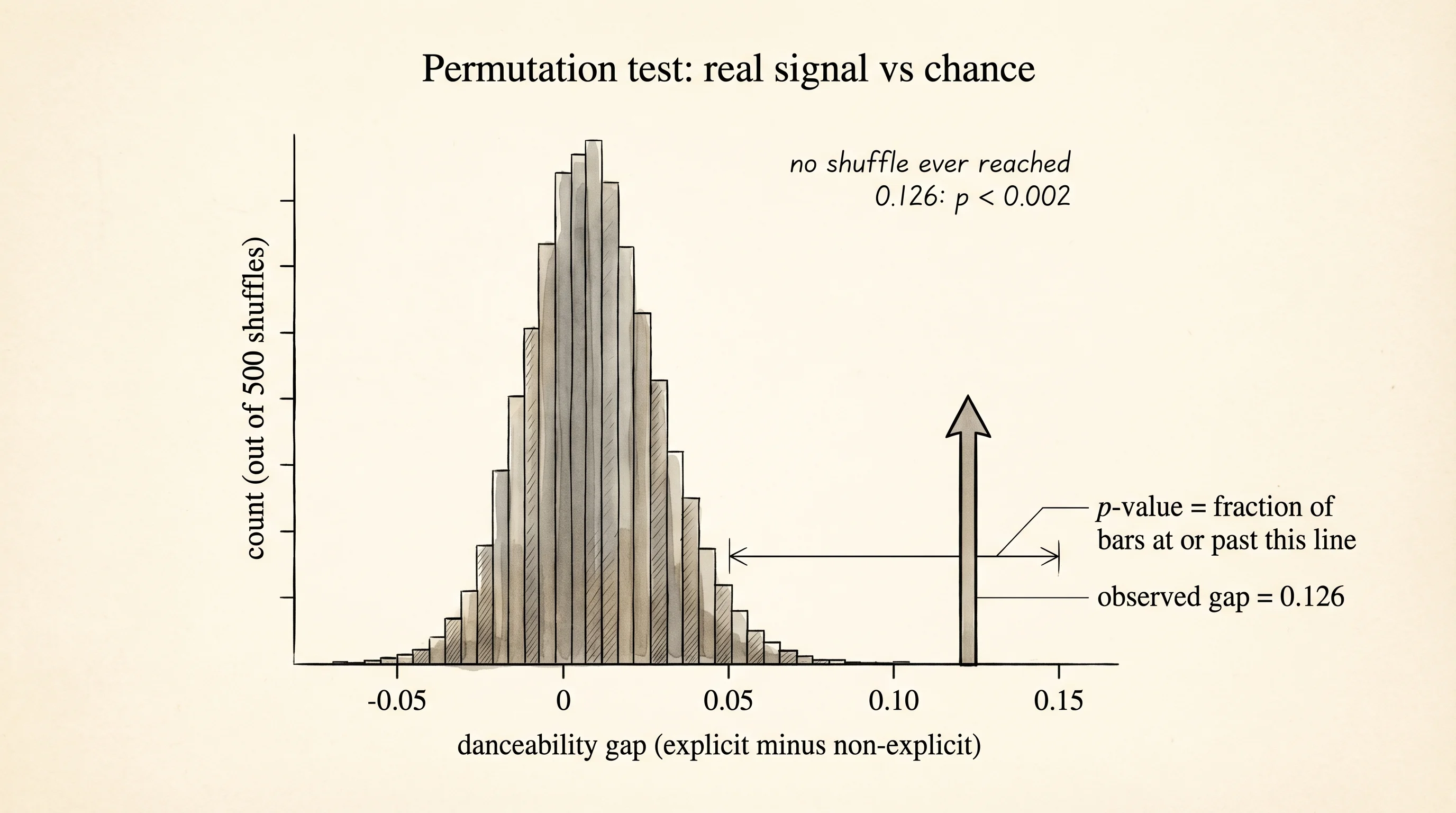
observed gap: 0.1262

The gap is 0.126. The p-value is the answer to: if there were no real difference between the two groups, how often would a gap at least this big show up by chance? The clean way to compute it without any imports is a permutation test, invented by Fisher himself. You throw all the danceability scores into one pile, ignore the labels, shuffle the pile, hand out new fake labels in the same group sizes, measure the gap, and repeat 1,000 times. The p-value is the fraction of those fake gaps that are at least as extreme as the real one.

import random
 
pooled = exp + safe
n_exp = len(exp)
 
random.seed(0)
extremes = 0
rounds = 500
for i in range(rounds):
    random.shuffle(pooled)
    fake_exp = pooled[:n_exp]
    fake_safe = pooled[n_exp:]
    fake_gap = sum(fake_exp) / n_exp - sum(fake_safe) / len(fake_safe)
    if abs(fake_gap) >= abs(observed_gap):
        extremes += 1
    if i < 5:
        print(f"round {i}: fake gap = {round(fake_gap, 4)}")
 
p_value = extremes / rounds
print("p-value:", p_value)

round 0: fake gap = -0.0012
round 1: fake gap = 0.0003
round 2: fake gap = 0.0008
round 3: fake gap = -0.0024
round 4: fake gap = -0.0009
p-value: 0.0

Every fake shuffle produced a gap near zero, never anywhere near 0.126. The p-value is 0 out of 500, which you report as p < 0.002. That means under the null hypothesis — the world where explicit and non-explicit tracks come from the same danceability distribution — a gap of 0.126 would happen less than 2 times in 1,000. It did not happen by luck. Explicit tracks are measurably more danceable, and the mechanism is the obvious one: hip-hop and pop dominate the explicit flag, and those genres are built around beats people dance to. Causation matches correlation here.

Run the same test on the fake finding from the last lesson — the even-year vs odd-year popularity gap of 0.183. The observed gap was small and the permutation test would give you a p-value above 0.05 almost every time, which is the standard line of "this looks like luck." The real correlation passes. The spurious one does not. That is the filter Fisher gave the world.

One more move. Bayesian thinking is the older way to ask the same kind of question. Instead of asking "how often would this happen by chance," you start with a prior — your belief about the world before you saw the data — and update it with each new piece of evidence. If your prior belief is that 10 percent of songs are explicit, and you pull a random song and see it has high danceability, Bayes's rule tells you exactly how much to nudge that 10 percent up or down. The formula is one line: posterior is proportional to prior times likelihood. The machinery behind every spam filter, every medical test interpretation, and every modern AI training loop is some version of that one line.

You can reason about your own data. Your laptop cannot stay on 24/7 to serve it to anyone else, and the moment you want two programs on two machines to talk, you need a protocol neither of them wrote.